Chapter – 1.
Production
and Cost

1.1
Production Function & Factors of Production

1)
What do
you mean by production

Production refers to the process of creating goods and services to satisfy
human wants. It involves converting inputs (like land, labour, capital)
into outputs (goods and services).

2) Define
a production function. What is its general mathematical form? (NCERT)

Meaning: The production function is a mathematical or functional
relationship between inputs (like land, labour, capital) and output
(finished goods/services).

🧾 General Form: Q = f (L, K) Where: Q = Output, L = Labour, K = Capital, f =
Function or relation

3) Distinguish
between fixed factors and variable factors of production. (MP 2022)

No.

Basis

Fixed Factors (cost)

Variable Factors (cost)

Meaning

Cost that does not change with output

Cost that changes with output

Example

Rent, salaries, interest

Raw materials, wages, electricity

Other name

Banded or supplementary costs or tied cost

Prime Costs, principal costs or direct costs or incremental
costs.

Output Relation

Same at all levels of output

Increases as output increases

Zero Output

Exists even if output is zero

Becomes zero when output is zero

Time Frame

Relevant in short run

Relevant in both short & long run

Diagram

4) What
is an isoquant? State two of its key properties. (NCERT)

shows
all possible combinations of two inputs (like labor and capital) that give same
level of output.

Property
1: An
isoquant slopes downward from left to right (negative slope) due to the
marginal rate of technical substitution.

Property
2: Higher
isoquants represent higher levels of output, and two isoquants never intersect
each other.

5) Explain
the Cobb-Douglas production function and its significance in economic analysis.

Ans: The Cobb-Douglas production
function is a specific functional form represented as

, It measures input-output
relationships in manufacturing industries. The sum of exponents (

) indicates returns to scale:

1.
if

, it exhibits Constant Returns to Scale;

2.
if

, Increasing Returns; and

3.
if

, Decreasing Returns.

6) Differentiate
between technological efficiency and economic efficiency in production.

S.No.

Basis

Technological Efficiency

Economic Efficiency

Meaning

Achieved when a firm
produces a given level of output using the minimum physical quantity of
inputs without waste.

Achieved when a firm
produces a given level of output at the absolute lowest monetary cost.

Focus

Physical transformation of
inputs into physical output.

Financial and monetary
cost minimization of inputs.

Dependency

Does not depend on input
market prices.

Directly depends on market
prices of inputs.

Example

Producing 100 units of
paper using the minimum possible wood pulp and power.

Choosing a combination of
labor and machinery that minimizes total wage and equipment costs for 100
units of paper.

7) Explain 4 factors of production:

These are the basic resources used to produce
goods and services.

1.
Land

Meaning: All natural resources used in production.
Examples: Soil, minerals, water, forests, sunlight.
Special Feature: It is fixed in supply and a free
gift of nature.

2. Labour

Meaning: Any human effort (physical or mental) used in production.
Examples: Farmer, teacher, factory worker.
Special Feature: Labour is perishable and cannot be
stored.

3. Capital

Meaning: All man-made resources used to produce other goods.
Examples: Tools, machinery, buildings, money.
Special Feature: Capital is produced means of production.

4. Enterprise (Entrepreneur)

Meaning: The person who organizes all other factors and takes the
risk.
Examples: Business owner, startup founder.
Special Feature: Bears risk and earns profit/loss.

Organisation (or Enterprise in some books)

Meaning: The coordination of land, labour, and capital to run a
business.

Test 3.1

1.
Which of the following is considered a
variable factor of production in the short run?

A) Factory Building     B)
Heavy Machinery    C) Raw
Materials        D) Permanent
Administrative Staff

2.
An equal-product curve representing different
combinations of two inputs yielding the same output level is called an
________.

3.
Explain the concept of production function.
Discuss the fundamental differences between short-run and long-run
production functions with appropriate examples.

Examples: Planning, decision-making, managing workers.

1.2
Short Run vs. Long Run

8) Distinguish
between the short run and long run production functions. (MP 2023)

No.

Basis

Short-Run Production
Function

Long-Run Production
Function

Meaning

A time period where at
least one factor of production is kept fixed while others are varied.

A time period where all
factors of production are variable and can be changed.

Factor Ratio

The ratio between fixed
and variable factors changes as output expands.

The ratio between
different inputs remains constant as all factors increase together.

Governing Law

Governed by the Law of
Variable Proportions (Returns to a Factor).

Governed by the Law of
Returns to Scale.

Example

Expanding crop yield by
adding more daily laborers on a fixed 5-acre piece of land.

Doubling factory size,
machinery count, and worker strength simultaneously to double output.

9) Why
is the distinction between short run and long run based on factor flexibility
rather than a fixed calendar duration?

The
distinction depends on how quickly a firm can adjust its production inputs, not
on a set calendar time. For an street food vendor, the long run may be a few
days to buy another cart, while for an steel manufacturing plant, acquiring
land and setting up heavy blast furnaces makes the short run last several
years.

Test 1.4

1.
In the long run, a production function exhibits which of the
following characteristics?

A) At least one factor is kept fixed B) All factors of production
are variable

C) Factor ratios constantly change D) Fixed cost remains
positive

2. The production law applicable in the short run
is called the Law of ________.

3. Explain why the short run involves both
fixed and variable factors, while all factors become variable in the long
run. Illustrate with an example from a manufacturing industry.

The
difference between the revenue and cost is called the firm’s profit

1.3
Product Concepts: TP, AP, and MP

10)
Define Total Product (TP), Average Product (AP),
and Marginal Product (MP). (NCERT)

Total
Product (TP):
The total physical output produced by a firm using a given quantity of variable
inputs combined with fixed inputs over a period.

Average
Product (AP):
Output produced per unit of variable factor employed.

Marginal
Product (MP):
The addition made to Total Product by employing one additional unit of the
variable input.

11)
Distinguish between Average Product (AP) and
Marginal Product (MP).

S.No.

Basis

Average Product (AP)

Marginal Product (MP)

Meaning

Total output produced per
unit of the variable factor used.

Additional output produced
by employing one more unit of the variable factor.

Formula

Zero / Negative Value

AP is always positive as
long as TP is positive; it can never be zero or negative.

MP can be positive, zero,
or negative.

Example

If 5 workers produce 50
units of output,

units per worker.

If 6 workers produce 58
units, the

of the 6th worker is

units.

12)
Explain the mathematical and graphical
relationships between Total Product (TP) and Marginal Product (MP). (NCERT)

1.
When MP increases, TP increases at an increasing rate.

2.
When MP falls but remains positive, TP increases at a decreasing rate
(reaches its maximum when

).

3.
When MP becomes negative, TP begins to decline.

13)
Explain the relationship between Average Product
(AP) and Marginal Product (MP). (NCERT)

As long as

, AP rises.
When

, AP is at its maximum point (MP cuts AP at its peak).
When

, AP falls.

14)
Complete the following table:

Variable Input (L)

Total Product (TP)

Average Product (AP)

Marginal Product (MP)

-8

Answer:
For

:

,

.

For

:

,

,

.
For

:

,

,

.
For

:

,

,

.
For

:

,

,

.

Quick
assessment: 3.2

1.
When Total Product (TP) reaches its maximum point, Marginal
Product (MP) is:

A) Positive and maximum B) Equal to
Average Product C) Zero D) Negative

2. Marginal product
curve cuts the average product curve at its ________ point.

3. Using a schedule
and diagram, explain the three-stage relationship between Total
Product (TP) and Marginal Product (MP).

For

:

,

,

.

1.4
Law of Variable Proportions (Law of Diminishing
Marginal Product)

15)
State the Law of Variable Proportions. (MP 2024)

Ans:The Law of Variable
Proportions states that as more and more units of a variable factor are
combined with fixed factors of production, the total product initially
increases at an increasing rate, then increases at a diminishing rate, and
finally begins to decline.

16)
What are the key assumptions underlying the Law
of Variable Proportions? (NCERT)

1.
The state of technology remains constant.

2.
At least one factor of production is kept fixed while others are varied.

3.
All units of the variable factor are homogeneous in quality and
efficiency.

4.
Input factors are combined in variable proportions.

17)
Distinguish between Stage 1, Stage 2, and Stage
3 of the Law of Variable Proportions.

No.

Basis

Stage 1: Increasing
Returns

Stage 2: Diminishing
Returns

Stage 3: Negative Returns

Meaning

Stage where Total Product
increases at an increasing rate.

Stage where Total Product
increases at a decreasing rate.

Stage where Total Product
starts declining.

Behavior of MP

Marginal Product increases
continuously and reaches its maximum.

Marginal Product starts
falling but remains positive until it reaches zero.

Marginal Product becomes
negative.

Behavior of TP

Total Product increases at
an increasing rate.

Total Product increases at
a decreasing rate and reaches its maximum.

Total Product declines.

Rational Producer Choice

Producer does not stop
here as fixed factors are underutilized.

Rational producer operates
in this stage as total output is maximized.

Producer never operates
here as extra labor reduces total output.

Example

Adding 1st and 2nd worker
where specialization speeds up production per worker.

Adding 3rd and 4th worker
where limited machinery causes each worker to add less extra output.

Adding 6th worker where
excessive crowding leads to operational chaos and lower total output.

18)
Explain the Law of Variable Proportions with the
help of a schedule and diagram. (MP 2020, MP 2023)

Fixed Input (K)

Variable Input (L)

Total Product (TP)

Marginal Product (MP)

Stage of Production

1 Unit

Stage 1: Increasing Returns

1 Unit

Stage 2: Diminishing Returns

1 Unit

-2

Stage 3: Negative Returns

Explanation
of Stages:

o
Stage 1 (Increasing Returns): TP grows at an increasing rate; MP rises to its peak
(6) due to better utilization of fixed factors.

o
Stage 2 (Diminishing Returns): TP grows at a decreasing rate; MP declines from 6 to
0. TP reaches maximum (16) when

.

Quick Assessment 4

A rational producer will always operate in which
stage of the Law of Variable Proportions?

A) Stage 1 (Increasing Returns) B)
Stage 2 (Diminishing Returns)

C) Stage 3 (Negative Returns) D)
Either Stage 1 or Stage 3

2. When Marginal Product is zero, Total
Product reaches its ________ level.

3. Explain the reasons behind the operation of
increasing returns, diminishing returns, and negative returns to a factor
in the short run.

Stage 3
(Negative Returns): TP starts falling from 16 to 14; MP becomes negative (-2) due to
over-crowding and inefficiency of variable inputs.

1.5
Returns to Scale

19)
Define Returns to Scale. (NCERT)

Ans:
Returns to
scale refers to the behavior of total output when all inputs (labor and
capital) are increased simultaneously in the exact same proportion in the long
run.

20)
Distinguish between Increasing, Constant, and
Decreasing Returns to Scale.

No.

Basis

Increasing Returns to
Scale (IRS)

Constant Returns to Scale
(CRS)

Decreasing Returns to
Scale (DRS)

Meaning

Output increases by a
greater percentage than the percentage increase in inputs.

Output increases by the
exact same percentage as the percentage increase in inputs.

Output increases by a
smaller percentage than the percentage increase in inputs.

Input-Output Relation

Cobb-Douglas Sum (

)

Primary Cause

Economies of scale
(internal and external advantages of bulk operations).

Balanced economies and
diseconomies of scale.

Diseconomies of scale
(management breakdown and coordination difficulties).

Example

Increasing all inputs by
100% causes total output to rise by 150%.

Doubling all factory
inputs results in exactly double the total output.

Doubling all inputs only
increases total production by 60% due to coordination issues.

21)
Distinguish between Returns to a Factor and
Returns to Scale. (MP 2022)

No.

Basis

Returns to a Factor

Returns to Scale

Meaning

Refers to changes in total
output when only one variable factor is changed while keeping other factors
fixed.

Refers to changes in total
output when all factors of production are changed in the same proportion.

Time Horizon

Operates exclusively in
the short run.

Operates exclusively in
the long run.

Factor Ratio

The ratio between fixed
and variable inputs constantly changes.

The ratio between
different production inputs remains constant.

Example

Increasing the number of
workers while keeping land size constant at 5 acres.

Doubling both land size
and worker strength at the exact same time.

22)
Explain how economies and diseconomies of scale
determine the shape of long-run output growth.

Quick Assessment 5

1.
If a firm increases all its inputs by 50% and
total output increases by 75%, the firm is experiencing:

A) Decreasing Returns to Scale B) Constant Returns to Scale

C) Increasing Returns to
Scale D) Diminishing Returns to a
Factor

2. Returns to scale operates only in the
________ run.

3. Explain the concept of Returns to Scale
using the Cobb-Douglas production function. Detail its three phases with
suitable numeric examples.

Ans: When a firm expands all
inputs, it initially experiences economies of scale (specialization,
better machinery utilization, bulk purchasing discounts), leading to Increasing
Returns to Scale. As expansion continues, economies equal diseconomies,
resulting in Constant Returns to Scale. If expansion goes beyond optimal
capacity, diseconomies of scale (communication gaps, supervisory
failure, managerial friction) dominate, resulting in Decreasing Returns to
Scale.

1.6
Cost Concepts & Short-Run Costs

23)
Define Total Fixed Cost (TFC), Total Variable
Cost (TVC), and Total Cost (TC). (NCERT)

Total
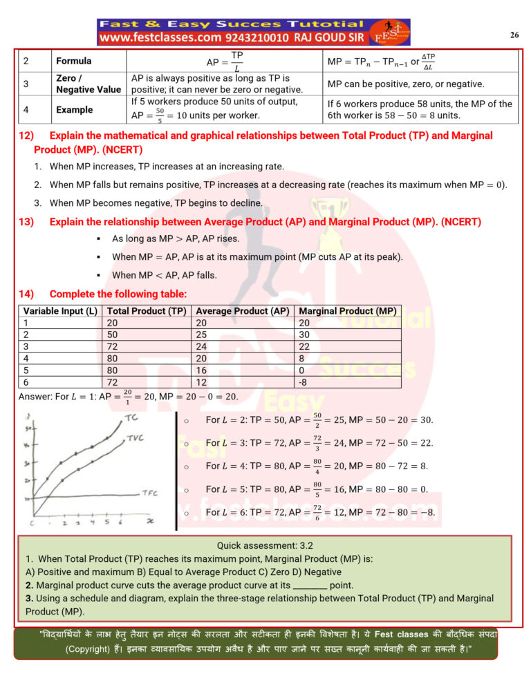
Fixed Cost (TFC): Costs incurred on fixed inputs that do not change with changes in
output quantity, even when output is zero.

Total
Variable Cost (TVC): Costs incurred on variable inputs that change directly with changes in
output levels.

Total
Cost (TC):
The total monetary expenditure incurred to produce a given quantity of output.

24)
Distinguish between Total Fixed Cost (TFC) and
Total Variable Cost (TVC). (MP 2022)

No.

Basis

Total Fixed Cost (TFC)

Total Variable Cost (TVC)

Meaning

Cost incurred on fixed
factors of production that remains constant regardless of output.

Cost incurred on variable
factors of production that changes directly with output level.

Value at Zero Output

Remains positive even when
output is zero (

).

Equals zero when total
output is zero (

).

Shape of Curve

Parallel to the horizontal
X-axis (horizontal straight line).

Inverted S-shaped curve
starting from the origin.

Example

Building rent, permanent
staff salaries, depreciation on heavy machinery.

Cost of raw materials,
electricity charges, daily wage labor wages.

25)
Distinguish between Average Cost (AC/SAC) and
Marginal Cost (MC/SMC).

S.No.

Basis

Average Cost (AC)

Marginal Cost (MC)

Meaning

Total cost per unit of
output produced.

Additional cost incurred
for producing one extra unit of output.

Formula

Minimum Point

Reaches its minimum after
MC reaches its minimum.

Reaches its minimum before
AC, and cuts AC from below at AC’s minimum point.

Example

If producing 5 units costs
₹50 in total,

per unit.

If total cost for 6 units
rises to ₹58, the MC of the 6th unit is

.

26)
Why is the Short-Run Average Cost (SAC) curve
‘U’-shaped? (NCERT)

The
SAC curve is ‘U’-shaped because of the Law of Variable Proportions:

1.
Initially (Falling Phase): As output expands, both Average Fixed Cost (AFC) and
Average Variable Cost (AVC) decline due to increasing returns to the variable
factor.

2.
At Optimum (Minimum Point): SAC reaches its lowest point where fixed factors are
fully utilized.

3.
Eventually (Rising Phase): Beyond optimum capacity, diminishing returns set in,
causing AVC (and consequently SAC) to rise rapidly.

27)

Quick Assessment 6

1. Which short-run cost curve continuously
declines as output increases but never touches the X-axis?

A) Short-Run Average
Cost (SAC) B) Average Fixed
Cost (AFC)

C) Average Variable Cost
(AVC) D) Short-Run
Marginal Cost (SMC)

2. The Marginal Cost (MC) curve intersects the
Average Cost (AC) curve at the ________ point of the AC curve.

3. Explain the relationship between Short-Run
Average Cost (SAC), Average Variable Cost (AVC), and Short-Run Marginal
Cost (SMC) using appropriate curves and diagrams.

Complete the following short-run cost table:

Output (q)

TFC

TVC

AFC

AVC

SAC

SMC

1.

stays constant at 60 across all
output levels.

3.

,

,

–

110

126

156

140

200

1.7
Long-Run Costs

28)
Define Long-Run Average Cost (LRAC) and Long-Run
Marginal Cost (LRMC). (NCERT)

1.
Long-Run Average Cost (LRAC): The total cost per unit of output when all inputs are
variable and the firm chooses the optimal scale of plant for each output level.

2.
Long-Run Marginal Cost (LRMC): The addition to long-run total cost resulting from
producing one additional unit of output when all inputs can be adjusted.

29)
Why is the Long-Run Average Cost (LRAC) curve
called an “Envelope Curve”?

Ans:
The LRAC
curve is composed of tangent points to a series of Short-Run Average Cost (SAC)
curves, each representing a different plant size. Because LRAC envelopes or
wraps around all possible short-run cost curves from below, it is known as an
“Envelope Curve” (or Planning Curve).

30)
Distinguish between Short-Run Average Cost (SAC)
and Long-Run Average Cost (LRAC).

No.

Basis

Short-Run Average Cost
(SAC)

Long-Run Average Cost
(LRAC)

Meaning

Per-unit cost of
production when at least one input factor is fixed.

Per-unit cost of
production when all inputs can be varied proportionally.

Fixed Cost Element

Includes both Average
Fixed Cost (AFC) and Average Variable Cost (AVC).

Consists only of variable
cost components as there are no fixed inputs in the long run.

Derivation

Derived directly from
short-run total cost curves.

Derived as an envelope
curve touching the lowest cost points of multiple SAC curves.

Example

Per-unit cost when
increasing output by running extra shifts in an existing factory.

Per-unit cost when
evaluating whether to double total plant capacity and open new facilities.

31)
Explain the shape of the LRAC curve in relation
to Returns to Scale. (NCERT)

The
LRAC curve is typically ‘U’-shaped due to long-run returns to scale:

1.
Falling Phase (Increasing Returns to Scale): As output expands
initially, economies of scale lower per-unit costs, causing LRAC to decline.

2.
Minimum Point (Constant Returns to Scale): LRAC reaches its minimum
point where economies equal diseconomies of scale (optimum firm size).

Quick Assessment 7

1. The Long-Run Average Cost curve is also
known as the:

A) Variable Curve B) Envelope Curve C) Marginal
Curve D) Fixed Cost Curve

2. In
the long run, total fixed cost is equal to ________.

3. Explain how the Long-Run Average Cost
(LRAC) curve is derived from Short-Run Average Cost (SAC) curves. Why does
LRAC decline initially and then rise?

Rising
Phase (Decreasing Returns to Scale): Beyond optimum output, diseconomies of scale
(managerial inefficiencies and coordination delays) cause LRAC to rise.

1.8
Other notes

tendency
of the MP to first increase and then fall is called the law of variable
proportions or the law of diminishing marginal product. Law of variable
proportions say that the marginal product of a factor input initially rises
with its employment level. But after reaching a certain level of employment, it
starts falling.

Average
cost

The cost per unit of an
item is called the average cost. Average Cost (AC) = Total Cost (TC) / Q

Types of average cost

Average fixed cost, Average
variable cost, Average total cost

Characteristics Average fixed cost:

1. It slopes downward to the right from left

2.

In the beginning, it slopes speedily and there after gradually It does
not touch the axis so it is in the shape of rectangular hyperbola: if we multiply the value of any point on the AFC curve
with the volume of production, the product obtained will be exactly the same as
multiplying its value at another point by the quantity produced.

3. It never become zero

4. Average Fixed Cost (AFC) = Total Fixed Cost (TFC) / Q

Average
variable cost

Average
Variable Cost (AVC) = Total Variable Cost (TVC) / Q And Average Cost (AC) = Total Cost (TC) / Q Thus, AC is the per-unit cost of
production. Diagrammatically, the vertical summation of average fixed cost
and average variable cost curves gives the short-run average cost curve.
SAC = TC/Q or SAC = AFC + AVC

Marginal Cost

Marginal cost
is the increase in the total cost resulting from one unit increase in
output. It may be called incremental cost.
Thus, MC = ΔTC/ΔQ.

Production

volume

Tied cost (₹)

TFC

Variable cost (₹)

Tvc

Total cost

Marginal cost

(MC)

–

Marginal cost is U shaped

Marginal cost
is the additional cost that a firm incurs to produce one extra unit of output.
According to the law of variable proportions, initially, the marginal product
of a factor increases as employment increases, and then after a certain point,
it decreases. This means initially to produce every extra unit of output, the
requirement of the factor becomes less and less, and then after a certain
point, it becomes greater and greater. As a result, with the factor price
given, initially the SMC falls, and then after a certain point, it rises. SMC
curve is, therefore, ‘U’-shaped.

Average cost is U shaped

Both SMC and
AVC curves start from the same point. Then, as output increases, SMC falls. AVC
being the average of marginal costs, also falls, but falls less than SMC. Then,
after a point, SMC starts rising. AVC, however, continues to fall as long as
the value of SMC remains less than the prevailing value of AVC. Once the SMC
has risen sufficiently, its value becomes greater than the value of AVC. The
AVC then starts rising. The AVC curve is therefore ‘U’-shaped.

As long as
AVC is falling, SMC must be less than the AVC. As AVC rises, SMC must be
greater than the AVC. So the SMC curve cuts the AVC curve from below at the
minimum point of AVC.

Short term average cost (SAC) is U shaped

SAC is the sum of AVC and
AFC. Initially, both AVC and AFC decrease as output increases. Therefore, SAC
initially falls. After a certain level of output production, AVC starts rising,
but AFC continuous to fall. Initially the fall in AFC is greater than the rise
in AVC and SAC is still falling. But, after a certain level of production, rise
in AVC becomes larger than the fall in AFC. From this point onwards, SAC is
rising. SAC curve is therefore ‘U’-shaped.

Quick assessment 8

1. When average cost rise marginal cost is ………..
the average cost

2. When average cost decline martinal cost is ……..
the average cost

3. Explain why marginal cost is U shaped

The U-shape of the Average Cost Curve reflects
that costs per unit fall in the beginning (due to economies of scale, better
resource use) and rise later (due to diseconomies and diminishing returns).Top of Form

MICRO ECONOMICS CHAPTER 3 PRODUCTION AND COST

Average cost

Types of average cost

Characteristics Average fixed cost:

Average variable cost

Marginal Cost

Marginal cost is U shaped

Average cost is U shaped

Short term average cost (SAC) is U shaped

Average
cost

Average
variable cost